
这是Andrej Karpathy 零基础学习神经网络的视频课的第三节课,在这一节课中,我们会实现一个简单的英文名生成网络。
准备工作
安装Python
安装Pytorch
观看视频课程
正式开始编写代码
准备姓名集和字典
首先,我们需要准备好姓名文本,这可以从GitHub上直接下载,读者可以点击直接下载进行下载。笔者已经把链接设置好了。
我们先按照上节课的思路,读取姓名集,并且创建字符映射整数索引的字典和反向字典:
import torch
import torch.nn.functional as F
import matplotlib.pyplot as plt

words = open("names.txt","r").read().splitlines()

chars = sorted(list(set("".join(words))))
stoi = { s : i+1 for i,s in enumerate(chars) } # 字符映射整数索引
stoi["."] = 0
itos = { i : s for s,i in stoi.items() } # 反向字典
print(stoi)
print(itos)
运行一下:
{'a': 1, 'b': 2, 'c': 3, 'd': 4, 'e': 5, 'f': 6, 'g': 7, 'h': 8, 'i': 9, 'j': 10, 'k': 11, 'l': 12, 'm': 13, 'n': 14, 'o': 15, 'p': 16, 'q': 17, 'r': 18, 's': 19, 't': 20, 'u': 21, 'v': 22, 'w': 23, 'x': 24, 'y': 25, 'z': 26, '.': 0}

{1: 'a', 2: 'b', 3: 'c', 4: 'd', 5: 'e', 6: 'f', 7: 'g', 8: 'h', 9: 'i', 10: 'j', 11: 'k', 12: 'l', 13: 'm', 14: 'n', 15: 'o', 16: 'p', 17: 'q', 18: 'r', 19: 's', 20: 't', 21: 'u', 22: 'v', 23: 'w', 24: 'x', 25: 'y', 26: 'z', 0: '.'}
准备训练样本
接下来我们需要准备训练用的样本,也就是输入什么、输出什么。我们的输入可以改为前面三个连续字符,而不是上一节课的前一个字符,输出就是第四个字符,当然这里的字符我们要用刚刚准备好的字典,映射为数字。我们重新写一个main.py:
import torch
import torch.nn.functional as F
import matplotlib.pyplot as plt

words = open("names.txt","r").read().splitlines()

# 创建字典和反向字典
chars = sorted(list(set("".join(words))))
stoi = { s : i+1 for i,s in enumerate(chars) } # 字符映射整数索引
stoi["."] = 0
itos = { i : s for s,i in stoi.items() } # 反向字典

block_size = 3
X, Y = [], []
for word in words[:1]:
    # 先在前面加上block_size个“.”,也就是加上若干个0,因为是按照stoi中的数字来保存的
    context = [0] * block_size
    for char in word + ".":
        ix = stoi[char]
        X.append(context)
        Y.append(ix)
        # 将context往后挪一个字符
        context = context[1:] + [ix]
        print(X)
        print(Y)
运行一下:
[[0, 0, 0]]
[5]
[[0, 0, 0], [0, 0, 5]]
[5, 13]
[[0, 0, 0], [0, 0, 5], [0, 5, 13]]
[5, 13, 13]
[[0, 0, 0], [0, 0, 5], [0, 5, 13], [5, 13, 13]]
[5, 13, 13, 1]
[[0, 0, 0], [0, 0, 5], [0, 5, 13], [5, 13, 13], [13, 13, 1]]
[5, 13, 13, 1, 0]
实现嵌入层
这是非常关键的一步,由于我们现在是通过前面三个字符来推导后面一个字符,如果我们还像上节课那样使用one_hot的方式向下一层传递样本的输入,那么这一层就需要27×3=81个输入,并且如果未来我们需要根据前5个、前10个字符来推导下一个字符的话,这里会变得更大,因此我们通过一个嵌入层将每一个字符转化为两个浮点数来表示。在这里我们想让每一个字符都有两个浮点数来表示,也就是一个嵌入层。
因为每一个字符都有两个浮点数来表示,所以它可以表达字符跟字符之间的位置关系。比如如果有两个字符在英文中有很多的共通点,那么它们的距离就会变得很近,反之则会变得很远。实际项目中,我们通常会使用50个甚至100个浮点数来表示一个字符或者一个词语。在这里我们为了方便演示,选择用2个浮点数的表示一个字符。
虽然一开始我们是随机的一个27×2的参数表,但是在未来通过反向传播,我们会逐渐地调整这个参数表更加准确。
C = torch.randn((27,2)) # 嵌入层
emb = C[torch.tensor(X)] # 将样本中的字符依次转化为浮点数表示
print(emb)
我们看一下输出:
tensor([[[ 1.0239, -0.8605],
         [ 1.0239, -0.8605],
         [ 1.0239, -0.8605]],

        [[ 1.0239, -0.8605],
         [ 1.0239, -0.8605],
         [ 0.4716,  0.6099]],

        [[ 1.0239, -0.8605],
         [ 0.4716,  0.6099],
         [ 0.1226,  0.3713]],

        [[ 0.4716,  0.6099],
         [ 0.1226,  0.3713],
         [ 0.1226,  0.3713]],

        [[ 0.1226,  0.3713],
         [ 0.1226,  0.3713],
         [ 0.2849, -1.1253]]])
实现隐藏层和输出层
可以看到,样本中的每一个字符都转换为了一个由两个浮点数表示的列表。下一步,将每一个样本中的这6个浮点数改为一个列表,输出给下一层隐藏层。这6个浮点数根据顺序依次排列,这样就可以体现出样本中字符的先后顺序。通过我们的这一步操作,原先需要将隐藏层传输81个输入,而现在我们只需要传入6个浮点数了,大大的减少了传入的量。
W1 = torch.randn((6,100))
b1 = torch.randn(100)

h = emb.view(-1,6) @ W1+b1
print(h.shape)emb.view(-1,6)这里的-1用于表示让PyTorch自行推导这里应该是多少。这里实际上是样本的数量,比如在现在它会推导出来是5,因为我们在刚刚只使用了姓名样本集中的最后一个姓名,的样本数量只有5。如果我们的样本有上万,那这个地方会推导出上万。
我们运行一下:
torch.Size([5, 100])可以看到,我们这一层给下一层神经网络提供了100个输出,那么下一个隐藏层就要提供100个输入。由于我们在这里只希望实现两层神经网络,因此,下一层神经网络要有27个输出,对应27个字符:
W2 = torch.randn((100,27))
b2 = torch.randn(27)
logits = h @ W2 + b2
print(logits.shape)
我们来运行一下:
torch.Size([5, 27])可以看到,我们输出层已经实现了27个输出。
固定随机种子
为了接下来更好的演示和复现,我修改了代码,固定了随机种子。以下是当前的完整代码:
import torch
import torch.nn.functional as F
import matplotlib.pyplot as plt

words = open("names.txt","r").read().splitlines()
g = torch.Generator().manual_seed(2147483647) # 固定随机种子

# 创建字典和反向字典
chars = sorted(list(set("".join(words))))
stoi = { s : i+1 for i,s in enumerate(chars) } # 字符映射整数索引
stoi["."] = 0
itos = { i : s for s,i in stoi.items() } # 反向字典

block_size = 3
X, Y = [], []
for word in words[:1]:
    # 先在前面加上block_size个“.”,也就是加上若干个0,因为是按照stoi中的数字来保存的
    context = [0] * block_size
    for char in word + ".":
        ix = stoi[char]
        X.append(context)
        Y.append(ix)
        # 将context往后挪一个字符
        context = context[1:] + [ix]

C = torch.randn((27,2), generator=g) # 嵌入层
emb = C[torch.tensor(X)] # 将样本中的字符依次转化为浮点数表示

# 第一层隐藏层
W1 = torch.randn((6,100), generator=g)
b1 = torch.randn(100, generator=g)
h = emb.view(-1,6) @ W1+b1

# 第二层输出层
W2 = torch.randn((100,27), generator=g)
b2 = torch.randn(27, generator=g)
logits = h @ W2 + b2
输出归一化与计算损失
接下来,我们再对输出层的输出进行归一化,并且计算损失:
counts = logits.exp()
prob = counts / counts.sum(1, keepdims=True)
loss = -prob[torch.arange(5),Y].log().mean()
当然,计算loss可以使用Pytorch的方法,我们无需重复造轮子:
loss = F.cross_entropy(logits, torch.tensor(Y))
print(loss)
运行一下:
tensor(99.6126)模型训练
接下来就是正向传播与反向传播,我们修改代码,让其能够进行微调的训练:
import torch
import torch.nn.functional as F
import matplotlib.pyplot as plt

words = open("names.txt","r").read().splitlines()
g = torch.Generator().manual_seed(2147483647) # 固定随机种子

# 创建字典和反向字典
chars = sorted(list(set("".join(words))))
stoi = { s : i+1 for i,s in enumerate(chars) } # 字符映射整数索引
stoi["."] = 0
itos = { i : s for s,i in stoi.items() } # 反向字典

block_size = 3
X, Y = [], []
for word in words[:5]:
    # 先在前面加上block_size个“.”,也就是加上若干个0,因为是按照stoi中的数字来保存的
    context = [0] * block_size
    for char in word + ".":
        ix = stoi[char]
        X.append(context)
        Y.append(ix)
        # 将context往后挪一个字符
        context = context[1:] + [ix]

C = torch.randn((27,2), generator=g) # 嵌入层

# 第一层隐藏层
W1 = torch.randn((6,100), generator=g)
b1 = torch.randn(100, generator=g)

# 第二层输出层
W2 = torch.randn((100,27), generator=g)
b2 = torch.randn(27, generator=g)

parameters = [C,W1,W2,b1,b2]
for p in parameters:
    p.requires_grad = True

for _ in range(100):
    emb = C[torch.tensor(X)]  # 将样本中的字符依次转化为浮点数表示
    h = emb.view(-1, 6) @ W1 + b1
    logits = h @ W2 + b2

    loss = F.cross_entropy(logits, torch.tensor(Y))
    for p in parameters:
        p.grad = None
    loss.backward()
    for p in parameters:
        p.data += -0.1 * p.grad
    print(loss.item())
让我们运行一下:
61.7388916015625
30.744335174560547
19.465017318725586
14.642541885375977
11.606647491455078
10.029589653015137
9.165127754211426
6.288736343383789
5.30631160736084
4.916451930999756
4.473801612854004
3.683753252029419
3.3870129585266113
3.616569995880127
5.824367523193359
6.791852951049805
3.6995389461517334
2.742274761199951
1.8824043273925781
1.9744515419006348
1.5300321578979492
1.6461244821548462
2.1655921936035156
3.659118175506592
2.467254161834717
1.3796861171722412
1.0965161323547363
1.2355493307113647
1.6014204025268555
1.3624526262283325
1.5353899002075195
1.307451605796814
1.1866517066955566
0.8342674374580383
0.875034749507904
0.8176398873329163
1.0066556930541992
1.0191515684127808
0.9441428780555725
0.6796780824661255
0.693280041217804
0.7197794914245605
0.733572781085968
0.6491024494171143
0.6743171215057373
0.6201052069664001
0.6231799125671387
0.5758059024810791
0.5589979887008667
0.5286083221435547
0.5157477259635925
0.49505743384361267
0.4789549708366394
0.46755141019821167
0.4543977975845337
0.44819700717926025
0.435586541891098
0.43247443437576294
0.4204025864601135
0.4189830422401428
0.40780332684516907
0.4070993661880493
0.397169828414917
0.396655797958374
0.3880215883255005
0.38747039437294006
0.37993234395980835
0.37929850816726685
0.3726232945919037
0.37193870544433594
0.3659595847129822
0.36525923013687134
0.3598758280277252
0.3591753840446472
0.3543221950531006
0.35362374782562256
0.3492506742477417
0.3485535681247711
0.3446139693260193
0.34391850233078003
0.34036877751350403
0.3396766483783722
0.3364769518375397
0.33578920364379883
0.33290255069732666
0.3322204351425171
0.3296143710613251
0.3289378881454468
0.3265831470489502
0.3259122669696808
0.32378315925598145
0.3231176435947418
0.32119160890579224
0.32053107023239136
0.3187873065471649
0.31813114881515503
0.3165515661239624
0.3158996105194092
0.3144682049751282
0.31382042169570923
可以看到我们的样本集只选用了前5个姓名,并且对于这个模型来说,它的损失值正在变小的。
近似梯度
样本集如果设定的是所有的样本一起计算的话,其计算的速度会很慢。因此我们可以使用近似梯度的方式加快计算过程。
近似梯度就是在样本集中随机拿取若干的样本,组成一个小的样本集,并且通过这个样本集去做前向传播和反向传播,计算梯度并进行训练,能够更快地达到更好的训练效果
使用近似梯度可以极大地加快我们的训练速度,但是由于每次计算出来的梯度并不是整个样本集的梯度,而是当前这个小样本级的梯度,所以我们需要增加训练次数来达到相同的效果
我们先修改代码,实现近似梯度训练:
import torch
import torch.nn.functional as F
import matplotlib.pyplot as plt

words = open("names.txt","r").read().splitlines()
g = torch.Generator().manual_seed(2147483647) # 固定随机种子

# 创建字典和反向字典
chars = sorted(list(set("".join(words))))
stoi = { s : i+1 for i,s in enumerate(chars) } # 字符映射整数索引
stoi["."] = 0
itos = { i : s for s,i in stoi.items() } # 反向字典

block_size = 3
X, Y = [], []
for word in words:
    # 先在前面加上block_size个“.”,也就是加上若干个0,因为是按照stoi中的数字来保存的
    context = [0] * block_size
    for char in word + ".":
        ix = stoi[char]
        X.append(context)
        Y.append(ix)
        # 将context往后挪一个字符
        context = context[1:] + [ix]

C = torch.randn((27,2), generator=g) # 嵌入层

# 第一层隐藏层
W1 = torch.randn((6,100), generator=g)
b1 = torch.randn(100, generator=g)

# 第二层输出层
W2 = torch.randn((100,27), generator=g)
b2 = torch.randn(27, generator=g)

parameters = [C,W1,W2,b1,b2]
X = torch.tensor(X)
Y = torch.tensor(Y)
for p in parameters:
    p.requires_grad = True

for _ in range(1000):

    ix = torch.randint(0,X.shape[0],(32,))
    emb = C[X[ix]]  # 将样本中的字符依次转化为浮点数表示

    h = emb.view(-1, 6) @ W1 + b1
    logits = h @ W2 + b2
    loss = F.cross_entropy(logits, Y[ix])
    for p in parameters:
        p.grad = None
    loss.backward()
    for p in parameters:
        p.data += -0.1 * p.grad
    print(loss.item())
运行一下:
49.284637451171875
42.29495620727539
32.57741165161133
31.870040893554688
21.491657257080078
17.07381248474121
16.543869018554688
......
2.9590938091278076
2.8406906127929688
2.9868624210357666
2.538074016571045
可以看到,由于使用了近似梯度,因此每次选择的小样本集也是不一样的,所以我们会发现其损失值的变化趋势不一定每一次都是减少的。我们再增加一段代码来看看最终训练结果对于整体样本的损失值:
emb = C[X]
h = emb.view(-1, 6) @ W1 + b1
logits = h @ W2 + b2
loss = F.cross_entropy(logits, Y)
print(loss.item())
运行一下,我在这里就截取最后两次输出:
3.044374465942383
3.019815444946289
可以看到,在本次训练中,最后一次使用相似梯度训练的损失值是3.044,而对于所有样本集的损失值是3.019,可以看到其区别不是很大,代表了我们的训练还是比较成功的。
添加非线性激活函数
从数学上,两个线性变换叠加,本质上等价于一个线性变换,这意味着无论我们的网络多深,它都无法拟合非线性关系。因此,我们需要修改h:
h = torch.tanh(emb.view(-1, 6) @ W1 + b1) # 加上 tanh 非线性追踪更好的学习率
我们现在还需要来探究一下,学习率设置为多少比较合适。首先我们生成一个-3到0的线性列表,然后将其作为10的x次幂,这样就能获得一个指数增长的列表:
# 学习率区间
lre = torch.linspace(-3,0,1000)
lrs = 10**lre
print(lrs)
运行一下:
tensor([0.0010, 0.0010, 0.0010, 0.0010, 0.0010, 0.0010, 0.0010, 0.0010, 0.0011,
        0.0011, 0.0011, 0.0011, 0.0011, 0.0011, 0.0011, 0.0011, 0.0011, 0.0011,
        0.0011, 0.0011, 0.0011, 0.0012, 0.0012, 0.0012, 0.0012, 0.0012, 0.0012,
        0.0012, 0.0012, 0.0012, 0.0012, 0.0012, 0.0012, 0.0013, 0.0013, 0.0013,
        0.0013, 0.0013, 0.0013, 0.0013, 0.0013, 0.0013, 0.0013, 0.0013, 0.0014,
        0.0014, 0.0014, 0.0014, 0.0014, 0.0014, 0.0014, 0.0014, 0.0014, 0.0014,
        0.0015, 0.0015, 0.0015, 0.0015, 0.0015, 0.0015, 0.0015, 0.0015, 0.0015,
        0.0015, 0.0016, 0.0016, 0.0016, 0.0016, 0.0016, 0.0016, 0.0016, 0.0016,
        0.0016, 0.0017, 0.0017, 0.0017, 0.0017, 0.0017, 0.0017, 0.0017, 0.0017,
        0.0018, 0.0018, 0.0018, 0.0018, 0.0018, 0.0018, 0.0018, 0.0018, 0.0019,
        0.0019, 0.0019, 0.0019, 0.0019, 0.0019, 0.0019, 0.0019, 0.0020, 0.0020,
        0.0020, 0.0020, 0.0020, 0.0020, 0.0020, 0.0021, 0.0021, 0.0021, 0.0021,
        0.0021, 0.0021, 0.0021, 0.0022, 0.0022, 0.0022, 0.0022, 0.0022, 0.0022,
        0.0022, 0.0023, 0.0023, 0.0023, 0.0023, 0.0023, 0.0023, 0.0024, 0.0024,
        0.0024, 0.0024, 0.0024, 0.0024, 0.0025, 0.0025, 0.0025, 0.0025, 0.0025,
        0.0025, 0.0026, 0.0026, 0.0026, 0.0026, 0.0026, 0.0027, 0.0027, 0.0027,
        0.0027, 0.0027, 0.0027, 0.0028, 0.0028, 0.0028, 0.0028, 0.0028, 0.0029,
        0.0029, 0.0029, 0.0029, 0.0029, 0.0030, 0.0030, 0.0030, 0.0030, 0.0030,
        0.0031, 0.0031, 0.0031, 0.0031, 0.0032, 0.0032, 0.0032, 0.0032, 0.0032,
        0.0033, 0.0033, 0.0033, 0.0033, 0.0034, 0.0034, 0.0034, 0.0034, 0.0034,
        0.0035, 0.0035, 0.0035, 0.0035, 0.0036, 0.0036, 0.0036, 0.0036, 0.0037,
        0.0037, 0.0037, 0.0037, 0.0038, 0.0038, 0.0038, 0.0039, 0.0039, 0.0039,
        0.0039, 0.0040, 0.0040, 0.0040, 0.0040, 0.0041, 0.0041, 0.0041, 0.0042,
        0.0042, 0.0042, 0.0042, 0.0043, 0.0043, 0.0043, 0.0044, 0.0044, 0.0044,
        0.0045, 0.0045, 0.0045, 0.0045, 0.0046, 0.0046, 0.0046, 0.0047, 0.0047,
        0.0047, 0.0048, 0.0048, 0.0048, 0.0049, 0.0049, 0.0049, 0.0050, 0.0050,
        0.0050, 0.0051, 0.0051, 0.0051, 0.0052, 0.0052, 0.0053, 0.0053, 0.0053,
        0.0054, 0.0054, 0.0054, 0.0055, 0.0055, 0.0056, 0.0056, 0.0056, 0.0057,
        0.0057, 0.0058, 0.0058, 0.0058, 0.0059, 0.0059, 0.0060, 0.0060, 0.0060,
        0.0061, 0.0061, 0.0062, 0.0062, 0.0062, 0.0063, 0.0063, 0.0064, 0.0064,
        0.0065, 0.0065, 0.0066, 0.0066, 0.0067, 0.0067, 0.0067, 0.0068, 0.0068,
        0.0069, 0.0069, 0.0070, 0.0070, 0.0071, 0.0071, 0.0072, 0.0072, 0.0073,
        0.0073, 0.0074, 0.0074, 0.0075, 0.0075, 0.0076, 0.0076, 0.0077, 0.0077,
        0.0078, 0.0079, 0.0079, 0.0080, 0.0080, 0.0081, 0.0081, 0.0082, 0.0082,
        0.0083, 0.0084, 0.0084, 0.0085, 0.0085, 0.0086, 0.0086, 0.0087, 0.0088,
        0.0088, 0.0089, 0.0090, 0.0090, 0.0091, 0.0091, 0.0092, 0.0093, 0.0093,
        0.0094, 0.0095, 0.0095, 0.0096, 0.0097, 0.0097, 0.0098, 0.0099, 0.0099,
        0.0100, 0.0101, 0.0101, 0.0102, 0.0103, 0.0104, 0.0104, 0.0105, 0.0106,
        0.0106, 0.0107, 0.0108, 0.0109, 0.0109, 0.0110, 0.0111, 0.0112, 0.0112,
        0.0113, 0.0114, 0.0115, 0.0116, 0.0116, 0.0117, 0.0118, 0.0119, 0.0120,
        0.0121, 0.0121, 0.0122, 0.0123, 0.0124, 0.0125, 0.0126, 0.0127, 0.0127,
        0.0128, 0.0129, 0.0130, 0.0131, 0.0132, 0.0133, 0.0134, 0.0135, 0.0136,
        0.0137, 0.0137, 0.0138, 0.0139, 0.0140, 0.0141, 0.0142, 0.0143, 0.0144,
        0.0145, 0.0146, 0.0147, 0.0148, 0.0149, 0.0150, 0.0151, 0.0152, 0.0154,
        0.0155, 0.0156, 0.0157, 0.0158, 0.0159, 0.0160, 0.0161, 0.0162, 0.0163,
        0.0165, 0.0166, 0.0167, 0.0168, 0.0169, 0.0170, 0.0171, 0.0173, 0.0174,
        0.0175, 0.0176, 0.0178, 0.0179, 0.0180, 0.0181, 0.0182, 0.0184, 0.0185,
        0.0186, 0.0188, 0.0189, 0.0190, 0.0192, 0.0193, 0.0194, 0.0196, 0.0197,
        0.0198, 0.0200, 0.0201, 0.0202, 0.0204, 0.0205, 0.0207, 0.0208, 0.0210,
        0.0211, 0.0212, 0.0214, 0.0215, 0.0217, 0.0218, 0.0220, 0.0221, 0.0223,
        0.0225, 0.0226, 0.0228, 0.0229, 0.0231, 0.0232, 0.0234, 0.0236, 0.0237,
        0.0239, 0.0241, 0.0242, 0.0244, 0.0246, 0.0247, 0.0249, 0.0251, 0.0253,
        0.0254, 0.0256, 0.0258, 0.0260, 0.0261, 0.0263, 0.0265, 0.0267, 0.0269,
        0.0271, 0.0273, 0.0274, 0.0276, 0.0278, 0.0280, 0.0282, 0.0284, 0.0286,
        0.0288, 0.0290, 0.0292, 0.0294, 0.0296, 0.0298, 0.0300, 0.0302, 0.0304,
        0.0307, 0.0309, 0.0311, 0.0313, 0.0315, 0.0317, 0.0320, 0.0322, 0.0324,
        0.0326, 0.0328, 0.0331, 0.0333, 0.0335, 0.0338, 0.0340, 0.0342, 0.0345,
        0.0347, 0.0350, 0.0352, 0.0354, 0.0357, 0.0359, 0.0362, 0.0364, 0.0367,
        0.0369, 0.0372, 0.0375, 0.0377, 0.0380, 0.0382, 0.0385, 0.0388, 0.0390,
        0.0393, 0.0396, 0.0399, 0.0401, 0.0404, 0.0407, 0.0410, 0.0413, 0.0416,
        0.0418, 0.0421, 0.0424, 0.0427, 0.0430, 0.0433, 0.0436, 0.0439, 0.0442,
        0.0445, 0.0448, 0.0451, 0.0455, 0.0458, 0.0461, 0.0464, 0.0467, 0.0471,
        0.0474, 0.0477, 0.0480, 0.0484, 0.0487, 0.0491, 0.0494, 0.0497, 0.0501,
        0.0504, 0.0508, 0.0511, 0.0515, 0.0518, 0.0522, 0.0526, 0.0529, 0.0533,
        0.0537, 0.0540, 0.0544, 0.0548, 0.0552, 0.0556, 0.0559, 0.0563, 0.0567,
        0.0571, 0.0575, 0.0579, 0.0583, 0.0587, 0.0591, 0.0595, 0.0599, 0.0604,
        0.0608, 0.0612, 0.0616, 0.0621, 0.0625, 0.0629, 0.0634, 0.0638, 0.0642,
        0.0647, 0.0651, 0.0656, 0.0660, 0.0665, 0.0670, 0.0674, 0.0679, 0.0684,
        0.0688, 0.0693, 0.0698, 0.0703, 0.0708, 0.0713, 0.0718, 0.0723, 0.0728,
        0.0733, 0.0738, 0.0743, 0.0748, 0.0753, 0.0758, 0.0764, 0.0769, 0.0774,
        0.0780, 0.0785, 0.0790, 0.0796, 0.0802, 0.0807, 0.0813, 0.0818, 0.0824,
        0.0830, 0.0835, 0.0841, 0.0847, 0.0853, 0.0859, 0.0865, 0.0871, 0.0877,
        0.0883, 0.0889, 0.0895, 0.0901, 0.0908, 0.0914, 0.0920, 0.0927, 0.0933,
        0.0940, 0.0946, 0.0953, 0.0959, 0.0966, 0.0973, 0.0979, 0.0986, 0.0993,
        0.1000, 0.1007, 0.1014, 0.1021, 0.1028, 0.1035, 0.1042, 0.1050, 0.1057,
        0.1064, 0.1072, 0.1079, 0.1087, 0.1094, 0.1102, 0.1109, 0.1117, 0.1125,
        0.1133, 0.1140, 0.1148, 0.1156, 0.1164, 0.1172, 0.1181, 0.1189, 0.1197,
        0.1205, 0.1214, 0.1222, 0.1231, 0.1239, 0.1248, 0.1256, 0.1265, 0.1274,
        0.1283, 0.1292, 0.1301, 0.1310, 0.1319, 0.1328, 0.1337, 0.1346, 0.1356,
        0.1365, 0.1374, 0.1384, 0.1394, 0.1403, 0.1413, 0.1423, 0.1433, 0.1443,
        0.1453, 0.1463, 0.1473, 0.1483, 0.1493, 0.1504, 0.1514, 0.1525, 0.1535,
        0.1546, 0.1557, 0.1567, 0.1578, 0.1589, 0.1600, 0.1611, 0.1623, 0.1634,
        0.1645, 0.1657, 0.1668, 0.1680, 0.1691, 0.1703, 0.1715, 0.1727, 0.1739,
        0.1751, 0.1763, 0.1775, 0.1788, 0.1800, 0.1812, 0.1825, 0.1838, 0.1850,
        0.1863, 0.1876, 0.1889, 0.1902, 0.1916, 0.1929, 0.1942, 0.1956, 0.1969,
        0.1983, 0.1997, 0.2010, 0.2024, 0.2038, 0.2053, 0.2067, 0.2081, 0.2096,
        0.2110, 0.2125, 0.2140, 0.2154, 0.2169, 0.2184, 0.2200, 0.2215, 0.2230,
        0.2246, 0.2261, 0.2277, 0.2293, 0.2309, 0.2325, 0.2341, 0.2357, 0.2373,
        0.2390, 0.2406, 0.2423, 0.2440, 0.2457, 0.2474, 0.2491, 0.2508, 0.2526,
        0.2543, 0.2561, 0.2579, 0.2597, 0.2615, 0.2633, 0.2651, 0.2669, 0.2688,
        0.2707, 0.2725, 0.2744, 0.2763, 0.2783, 0.2802, 0.2821, 0.2841, 0.2861,
        0.2880, 0.2900, 0.2921, 0.2941, 0.2961, 0.2982, 0.3002, 0.3023, 0.3044,
        0.3065, 0.3087, 0.3108, 0.3130, 0.3151, 0.3173, 0.3195, 0.3217, 0.3240,
        0.3262, 0.3285, 0.3308, 0.3331, 0.3354, 0.3377, 0.3400, 0.3424, 0.3448,
        0.3472, 0.3496, 0.3520, 0.3544, 0.3569, 0.3594, 0.3619, 0.3644, 0.3669,
        0.3695, 0.3720, 0.3746, 0.3772, 0.3798, 0.3825, 0.3851, 0.3878, 0.3905,
        0.3932, 0.3959, 0.3987, 0.4014, 0.4042, 0.4070, 0.4098, 0.4127, 0.4155,
        0.4184, 0.4213, 0.4243, 0.4272, 0.4302, 0.4331, 0.4362, 0.4392, 0.4422,
        0.4453, 0.4484, 0.4515, 0.4546, 0.4578, 0.4610, 0.4642, 0.4674, 0.4706,
        0.4739, 0.4772, 0.4805, 0.4838, 0.4872, 0.4906, 0.4940, 0.4974, 0.5008,
        0.5043, 0.5078, 0.5113, 0.5149, 0.5185, 0.5221, 0.5257, 0.5293, 0.5330,
        0.5367, 0.5404, 0.5442, 0.5479, 0.5517, 0.5556, 0.5594, 0.5633, 0.5672,
        0.5712, 0.5751, 0.5791, 0.5831, 0.5872, 0.5913, 0.5954, 0.5995, 0.6036,
        0.6078, 0.6120, 0.6163, 0.6206, 0.6249, 0.6292, 0.6336, 0.6380, 0.6424,
        0.6469, 0.6513, 0.6559, 0.6604, 0.6650, 0.6696, 0.6743, 0.6789, 0.6837,
        0.6884, 0.6932, 0.6980, 0.7028, 0.7077, 0.7126, 0.7176, 0.7225, 0.7275,
        0.7326, 0.7377, 0.7428, 0.7480, 0.7531, 0.7584, 0.7636, 0.7689, 0.7743,
        0.7796, 0.7850, 0.7905, 0.7960, 0.8015, 0.8071, 0.8127, 0.8183, 0.8240,
        0.8297, 0.8355, 0.8412, 0.8471, 0.8530, 0.8589, 0.8648, 0.8708, 0.8769,
        0.8830, 0.8891, 0.8953, 0.9015, 0.9077, 0.9140, 0.9204, 0.9268, 0.9332,
        0.9397, 0.9462, 0.9528, 0.9594, 0.9660, 0.9727, 0.9795, 0.9863, 0.9931,
        1.0000])
接下来我们修改代码,保存不同的学习率对损失造成的影响:
import torch
import torch.nn.functional as F
import matplotlib.pyplot as plt

words = open("names.txt","r").read().splitlines()
g = torch.Generator().manual_seed(2147483647) # 固定随机种子

# 创建字典和反向字典
chars = sorted(list(set("".join(words))))
stoi = { s : i+1 for i,s in enumerate(chars) } # 字符映射整数索引
stoi["."] = 0
itos = { i : s for s,i in stoi.items() } # 反向字典

block_size = 3
X, Y = [], []
for word in words:
    # 先在前面加上block_size个“.”,也就是加上若干个0,因为是按照stoi中的数字来保存的
    context = [0] * block_size
    for char in word + ".":
        ix = stoi[char]
        X.append(context)
        Y.append(ix)
        # 将context往后挪一个字符
        context = context[1:] + [ix]

C = torch.randn((27,2), generator=g) # 嵌入层

# 第一层隐藏层
W1 = torch.randn((6,100), generator=g)
b1 = torch.randn(100, generator=g)

# 第二层输出层
W2 = torch.randn((100,27), generator=g)
b2 = torch.randn(27, generator=g)

parameters = [C,W1,W2,b1,b2]
X = torch.tensor(X)
Y = torch.tensor(Y)

# 学习率区间
lre = torch.linspace(-3,0,1000)
lrs = 10**lre
# print(lrs)

for p in parameters:
    p.requires_grad = True

lri = []
lossi = []

for i in range(1000):

    ix = torch.randint(0,X.shape[0],(32,))
    emb = C[X[ix]]  # 将样本中的字符依次转化为浮点数表示

    h = torch.tanh(emb.view(-1, 6) @ W1 + b1)
    logits = h @ W2 + b2
    loss = F.cross_entropy(logits, Y[ix])
    for p in parameters:
        p.grad = None
    loss.backward()

    lr = lrs[i]
    for p in parameters:
        p.data += -lr * p.grad

    lri.append(lre[i])
    lossi.append(loss.item())
    # print(loss.item())

emb = C[X]
h = torch.tanh(emb.view(-1, 6) @ W1 + b1)
logits = h @ W2 + b2
loss = F.cross_entropy(logits, Y)
# print(loss.item())

plt.plot(lri, lossi)
plt.xlabel('Learning Rate')
plt.ylabel('Loss')
plt.show()
运行一下:
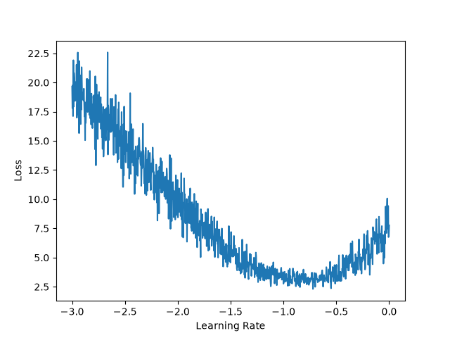
我们可以看到,学习率在-1处比较优秀,也就是10**-1=0.1。也就是说,我们最后得出结论,学习率设为0.1比较好
学习率衰减
因为一开始使用0.1的学习率可以获得较好的效果,但当训练次数更大,模型已经变得更精细的时候,我们可以对学习率进行衰减,比如衰减其为1/10,这样可以让我们的模型达到更好的效果:
import torch
import torch.nn.functional as F
import matplotlib.pyplot as plt

words = open("names.txt","r").read().splitlines()
g = torch.Generator().manual_seed(2147483647) # 固定随机种子

# 创建字典和反向字典
chars = sorted(list(set("".join(words))))
stoi = { s : i+1 for i,s in enumerate(chars) } # 字符映射整数索引
stoi["."] = 0
itos = { i : s for s,i in stoi.items() } # 反向字典

block_size = 3
X, Y = [], []
for word in words:
    # 先在前面加上block_size个“.”,也就是加上若干个0,因为是按照stoi中的数字来保存的
    context = [0] * block_size
    for char in word + ".":
        ix = stoi[char]
        X.append(context)
        Y.append(ix)
        # 将context往后挪一个字符
        context = context[1:] + [ix]

C = torch.randn((27,2), generator=g) # 嵌入层

# 第一层隐藏层
W1 = torch.randn((6,100), generator=g)
b1 = torch.randn(100, generator=g)

# 第二层输出层
W2 = torch.randn((100,27), generator=g)
b2 = torch.randn(27, generator=g)

parameters = [C,W1,W2,b1,b2]
X = torch.tensor(X)
Y = torch.tensor(Y)

for p in parameters:
    p.requires_grad = True

for i in range(200000):

    ix = torch.randint(0,X.shape[0],(32,))
    emb = C[X[ix]]  # 将样本中的字符依次转化为浮点数表示

    h = torch.tanh(emb.view(-1, 6) @ W1 + b1)
    logits = h @ W2 + b2
    loss = F.cross_entropy(logits, Y[ix])
    for p in parameters:
        p.grad = None
    loss.backward()

    lr = 0.1 if i < 100000 else 0.01
    for p in parameters:
        p.data += -lr * p.grad

    if i % 10000 == 0:
        print(loss.item())

emb = C[X]
h = torch.tanh(emb.view(-1, 6) @ W1 + b1)
logits = h @ W2 + b2
loss = F.cross_entropy(logits, Y)
print(loss.item())
运行一下:
18.17679786682129
2.4790353775024414
2.3036465644836426
2.5743117332458496
2.6201894283294678
2.1168222427368164
2.4747679233551025
2.5844204425811768
2.0612902641296387
2.0741043090820312
2.733124256134033
2.4877028465270996
2.463047504425049
2.0046935081481934
2.7823586463928223
2.194141387939453
1.9175939559936523
2.2526872158050537
2.0886881351470947
2.3008806705474854
2.2558350563049316
拆分样本集
我们可以把整个样本集拆分成训练集、验证集和测试集,分别占比80%10%和10%。现在让我们来实现一下,我们用训练集来训练,用验证集来检测最终的结果。由于我们目前实现的比较粗糙,没有通过验证集来决定学习率的高低,测试集反而没有用了。我们来实现一下:
import torch
import torch.nn.functional as F
import matplotlib.pyplot as plt
import random

words = open("names.txt","r").read().splitlines()
g = torch.Generator().manual_seed(2147483647) # 固定随机种子

# 创建字典和反向字典
chars = sorted(list(set("".join(words))))
stoi = { s : i+1 for i,s in enumerate(chars) } # 字符映射整数索引
stoi["."] = 0
itos = { i : s for s,i in stoi.items() } # 反向字典

def build_dataset(words):
    block_size = 3
    X, Y = [], []
    for word in words:
        # 先在前面加上block_size个“.”,也就是加上若干个0,因为是按照stoi中的数字来保存的
        context = [0] * block_size
        for char in word + ".":
            ix = stoi[char]
            X.append(context)
            Y.append(ix)
            # 将context往后挪一个字符
            context = context[1:] + [ix]
    X = torch.tensor(X)
    Y = torch.tensor(Y)
    print(X.shape, Y.shape)
    return X, Y

random.seed(42)
random.shuffle(words)
n1 = int(0.8*len(words))
n2 = int(0.9*len(words))
Xtr, Ytr = build_dataset(words[:n1])
Xdev, Ydev = build_dataset(words[n1:n2])
Xte, Yte = build_dataset(words[n2:])


C = torch.randn((27,2), generator=g) # 嵌入层

# 第一层隐藏层
W1 = torch.randn((6,100), generator=g)
b1 = torch.randn(100, generator=g)

# 第二层输出层
W2 = torch.randn((100,27), generator=g)
b2 = torch.randn(27, generator=g)

parameters = [C,W1,W2,b1,b2]


for p in parameters:
    p.requires_grad = True

for i in range(200000):

    ix = torch.randint(0,Xtr.shape[0],(32,))
    emb = C[Xtr[ix]]  # 将样本中的字符依次转化为浮点数表示

    h = torch.tanh(emb.view(-1, 6) @ W1 + b1)
    logits = h @ W2 + b2
    loss = F.cross_entropy(logits, Ytr[ix])
    for p in parameters:
        p.grad = None
    loss.backward()

    lr = 0.1 if i < 100000 else 0.01
    for p in parameters:
        p.data += -lr * p.grad

    if i % 10000 == 0:
        print(loss.item())

emb = C[Xdev]
h = torch.tanh(emb.view(-1, 6) @ W1 + b1)
logits = h @ W2 + b2
loss = F.cross_entropy(logits, Ydev)
print(loss.item())
运行一下:
torch.Size([182625, 3]) torch.Size([182625])
torch.Size([22655, 3]) torch.Size([22655])
torch.Size([22866, 3]) torch.Size([22866])
20.83146095275879
2.6087646484375
2.931648015975952
2.515237808227539
2.7970528602600098
2.529646396636963
2.2188212871551514
2.567169189453125
2.2405734062194824
2.0721330642700195
2.15317440032959
2.5734517574310303
1.836839199066162
2.461702346801758
2.326200008392334
2.4253039360046387
2.2661197185516357
1.8648080825805664
2.230231523513794
2.241915225982666
2.2516772747039795
可以看到,在训练集中训练的最后一次损失是2.2419,而在验证集上进行验证的损失值是2.2516,还是比较接近的。
优化损失值
目前损失值被我们压到了2.25左右。我们可以通过增大嵌入层的维数,和增加中间隐藏层的神经元数量,让我们的模型的损失值更加低:
import torch
import torch.nn.functional as F
import matplotlib.pyplot as plt
import random

words = open("names.txt","r").read().splitlines()
g = torch.Generator().manual_seed(2147483647) # 固定随机种子

# 创建字典和反向字典
chars = sorted(list(set("".join(words))))
stoi = { s : i+1 for i,s in enumerate(chars) } # 字符映射整数索引
stoi["."] = 0
itos = { i : s for s,i in stoi.items() } # 反向字典
block_size = 3

def build_dataset(words):
    X, Y = [], []
    for word in words:
        # 先在前面加上block_size个“.”,也就是加上若干个0,因为是按照stoi中的数字来保存的
        context = [0] * block_size
        for char in word + ".":
            ix = stoi[char]
            X.append(context)
            Y.append(ix)
            # 将context往后挪一个字符
            context = context[1:] + [ix]
    X = torch.tensor(X)
    Y = torch.tensor(Y)
    print(X.shape, Y.shape)
    return X, Y

random.seed(42)
random.shuffle(words)
n1 = int(0.8*len(words))
n2 = int(0.9*len(words))
Xtr, Ytr = build_dataset(words[:n1])
Xdev, Ydev = build_dataset(words[n1:n2])
Xte, Yte = build_dataset(words[n2:])

c_size = 30
C = torch.randn((27,c_size), generator=g) # 嵌入层

# 第一层隐藏层
W1 = torch.randn((c_size*block_size,500), generator=g)
b1 = torch.randn(500, generator=g)

# 第二层输出层
W2 = torch.randn((500,27), generator=g)
b2 = torch.randn(27, generator=g)

parameters = [C,W1,W2,b1,b2]


for p in parameters:
    p.requires_grad = True

for i in range(200000):

    ix = torch.randint(0,Xtr.shape[0],(32,))
    emb = C[Xtr[ix]]  # 将样本中的字符依次转化为浮点数表示

    h = torch.tanh(emb.view(-1, c_size*block_size) @ W1 + b1)
    logits = h @ W2 + b2
    loss = F.cross_entropy(logits, Ytr[ix])
    for p in parameters:
        p.grad = None
    loss.backward()

    lr = 0.1 if i < 100000 else 0.01
    for p in parameters:
        p.data += -lr * p.grad

    if i % 10000 == 0:
        print(loss.item())

emb = C[Xdev]
h = torch.tanh(emb.view(-1, c_size*block_size) @ W1 + b1)
logits = h @ W2 + b2
loss = F.cross_entropy(logits, Ydev)
print(loss.item())
运行一下:
D:\Data\Anacondea\envs\lora\python.exe D:\Data\Python\Class_3\main.py
torch.Size([182625, 3]) torch.Size([182625])
torch.Size([22655, 3]) torch.Size([22655])
torch.Size([22866, 3]) torch.Size([22866])
41.01119613647461
2.6473662853240967
3.1581287384033203
2.8194284439086914
3.114468574523926
2.694441795349121
2.2945523262023926
2.6995344161987305
2.6593563556671143
3.0314278602600098
2.737340211868286
1.6961545944213867
1.9784475564956665
2.1313881874084473
2.1206936836242676
1.9203801155090332
2.08767032623291
1.915178894996643
2.2067370414733887
1.9190465211868286
2.1798207759857178
可以看到,我们的损失值已经被降到2.1798了,甚至很多时候能降到2以下。
让模型输出
最后我们实现一个方法,让训练好的模型进行输出,以下是最终完整代码:
import torch
import torch.nn.functional as F
import matplotlib.pyplot as plt
import random

words = open("names.txt","r").read().splitlines()
g = torch.Generator().manual_seed(2147483647) # 固定随机种子

# 创建字典和反向字典
chars = sorted(list(set("".join(words))))
stoi = { s : i+1 for i,s in enumerate(chars) } # 字符映射整数索引
stoi["."] = 0
itos = { i : s for s,i in stoi.items() } # 反向字典
block_size = 3

def build_dataset(words):
    X, Y = [], []
    for word in words:
        # 先在前面加上block_size个“.”,也就是加上若干个0,因为是按照stoi中的数字来保存的
        context = [0] * block_size
        for char in word + ".":
            ix = stoi[char]
            X.append(context)
            Y.append(ix)
            # 将context往后挪一个字符
            context = context[1:] + [ix]
    X = torch.tensor(X)
    Y = torch.tensor(Y)
    print(X.shape, Y.shape)
    return X, Y

random.seed(42)
random.shuffle(words)
n1 = int(0.8*len(words))
n2 = int(0.9*len(words))
Xtr, Ytr = build_dataset(words[:n1])
Xdev, Ydev = build_dataset(words[n1:n2])
Xte, Yte = build_dataset(words[n2:])

c_size = 30
C = torch.randn((27,c_size), generator=g) # 嵌入层

# 第一层隐藏层
W1 = torch.randn((c_size*block_size,500), generator=g)
b1 = torch.randn(500, generator=g)

# 第二层输出层
W2 = torch.randn((500,27), generator=g)
b2 = torch.randn(27, generator=g)

parameters = [C,W1,W2,b1,b2]


for p in parameters:
    p.requires_grad = True

for i in range(200000):

    ix = torch.randint(0,Xtr.shape[0],(32,))
    emb = C[Xtr[ix]]  # 将样本中的字符依次转化为浮点数表示

    h = torch.tanh(emb.view(-1, c_size*block_size) @ W1 + b1)
    logits = h @ W2 + b2
    loss = F.cross_entropy(logits, Ytr[ix])
    for p in parameters:
        p.grad = None
    loss.backward()

    lr = 0.1 if i < 100000 else 0.01
    for p in parameters:
        p.data += -lr * p.grad

    if i % 10000 == 0:
        print(loss.item())

emb = C[Xdev]
h = torch.tanh(emb.view(-1, c_size*block_size) @ W1 + b1)
logits = h @ W2 + b2
loss = F.cross_entropy(logits, Ydev)
print(loss.item())

for _ in range(20):
    out = []
    context = [0] * block_size
    while True:
        emb = C[torch.tensor([context])]
        h = torch.tanh(emb.view(1, c_size*block_size) @ W1 + b1)
        logits = h @ W2 + b2
        probs = F.softmax(logits, dim=1)
        ix = torch.multinomial(probs, num_samples=1, generator=g).item()
        context = context[1:] + [ix]
        out.append(ix)
        if ix ==0 :
            break

    print("".join(itos[i] for i in out))
运行一下:
torch.Size([182625, 3]) torch.Size([182625])
torch.Size([22655, 3]) torch.Size([22655])
torch.Size([22866, 3]) torch.Size([22866])
45.05998611450195
4.614674091339111
2.5040812492370605
3.028714656829834
3.449761390686035
2.4731736183166504
2.022644281387329
2.3816988468170166
2.354505777359009
1.9231696128845215
2.955782413482666
1.9705157279968262
2.3768727779388428
1.6785004138946533
2.2360496520996094
2.1877331733703613
2.0761871337890625
2.1870200634002686
2.045487403869629
1.9190195798873901
2.1788113117218018
forkelshan.
charry.
kaliquella.
milyansh.
kail.
alania.
saman.
iriousratilee.
kearonxomitaliq.
awazem.
lamrahire.
grahira.
re.
trackin.
kau.
rubi.
ama.
leahneud.
graesyn.
ges.
结语
在这一节课中,我们训练的模型不是只通过上一个字符推导下一个字符,而是通过前三个字符推导后一个字符,其损失率已经降到了2.45以下,达到了2.17左右,取得了较大的进步,并且输出的也更像一个正常的英文名字了。当然这里还优化的地方,包括对学习率进行优化,对嵌层的维度进行优化,对隐藏层的神经元数量进行优化等。